QUICKER HIRE

News Classification: An NLP Exercise with LSTM

Here, we will try to classify Bangla news contents with an LSTM network. Bangla is a diverse and complex language. The dataset contains 400k+ Bangla news samples of 25+ categories. We will reach 91% test accuracy for our simple LSTM model.

We have text data (news contents) in utf-8 format, let's import the libraries and the data which is in JSON file. For each news content, we have a corresponding label - which we'll try to predict. So, this a text classification problem.

import numpy as np
import pandas as pd
import matplotlib.pyplot as plt


import pickle
from collections import Counter

In [3]:

import json
with open('data.json', encoding='utf-8') as fh:
    data = json.load(fh)

Figure: LSTM layer, it consists of multiple gates which is responsible for memory. Credit: Wikimedia

{'author': 'গাজীপুর প্রতিনিধি', 'category': 'bangladesh', 'category_bn': 'বাংলাদেশ', 'published_date': '০৪ জুলাই ২০১৩, ২৩:২৬', 'modification_date': '০৪ জুলাই ২০১৩, ২৩:২৭', 'tag': ['গাজীপুর'], 'comment_count': 0, 'title': 'কালিয়াকৈরে টিফিন খেয়ে ৫০০ শ্রমিক অসুস্থ, বিক্ষোভ', 'url': 'http://www.prothom-alo.com/bangladesh/article/19030', 'content': '...'}

This is a sample data point schema. There are multiple attributes we can see like author, category, published_date; but we're only concerned with category and content attributes. We'll be using an LSTM network for the classification task.

z = zip(cat_cnts, set_cats)
z = list(z)

[(83, 'nagorik-kantho'),
 (859, 'special-supplement'),
 (7402, 'durporobash'),
 (1, 'bs-events'),
 (508, 'kishoralo'),
 (15699, 'opinion'),
 (2, 'events'),
 (990, 'bondhushava'),
 (11, '22221'),
 (49012, 'sports'),
 (1, 'AskEditor'),
 (10, 'facebook'),
 (17, 'mpaward1'),
 (6990, 'northamerica'),
 (40, 'tarunno'),
 (10852, 'life-style'),
 (3443, 'pachmisheli'),
 (123, '-1'),
 (30856, 'international'),
 (232504, 'bangladesh'),
 (2604, 'roshalo'),
 (17245, 'economy'),
 (2999, 'we-are'),
 (75, 'chakri-bakri'),
 (9721, 'education'),
 (30466, 'entertainment'),
 (2702, 'onnoalo'),
 (2, 'diverse'),
 (443, 'trust'),
 (170, 'protichinta'),
 (2, 'demo-content'),
 (12116, 'technology')]

Here, we have frequency of each class. There are some classes with too few examples, let's remove them and focus only on the important ones.

sel_cats = []

for p in z:if p[0] > 8000:sel_cats.append(p[1])

sel_cats

['opinion',
 'sports',
 'life-style',
 'international',
 'bangladesh',
 'economy',
 'education',
 'entertainment',
 'technology']

So, we have 9 classes now. The randomized accuracy is 11.11%. Let's see how better we can do.

X_text = []
y_label = []

for p in data:
  if p['category'] in sel_cats:
    y_label.append(p['category'])
    X_text.append(p['content'])

len(X_text)

len(y_label)

Let's encode the text labels to numeric labels with LabelEncoder.

from sklearn.preprocessing import LabelEncoder

encoder = LabelEncoder()
class_labels = encoder.fit_transform(y_label)

From the numeric labels, we will generate the one-hot vector for multi-class classification.

from sklearn.preprocessing import OneHotEncoder

encoder = OneHotEncoder(sparse=False)
class_labels = class_labels.reshape((class_labels.shape[0], 1))
y_ohe = encoder.fit_transform(class_labels)

Now, we need to pre-process the text data to tokenized form.

from keras.preprocessing.text import Tokenizer

tokenizer = Tokenizer()
tokenizer.fit_on_texts(X_text)

X_token = tokenizer.texts_to_sequences(X_text)

vocab_size = len(tokenizer.word_index) + 1  # Adding 1 because of reserved 0 index

We will also be using post padding so that each news content has the same length.

from keras.preprocessing.sequence import pad_sequences
maxlen = 300
X_pad = pad_sequences(X_token, padding='post', maxlen=maxlen)

Here, each of the input text will be converted to a length 300 vector.

As, the dataset is imbalanced we'll also use class weight in terms of inverse frequency.

class_weight = {}

for c in (list(c_l)):

print(c)

c_w = len(class_labels)/np.sum(class_labels==c)

print(c_w)

class_weight[c] = c_w

Finally, let's design our simple LSTM network with Keras.

from keras.models import Sequential
from keras.layers import Embedding, CuDNNLSTM, Bidirectional, Dense

embedding_dim = 8

model = Sequential()
model.add(Embedding(input_dim=vocab_size, 
                           output_dim=embedding_dim, 
                           input_length=maxlen))
model.add(Bidirectional(CuDNNLSTM(128, return_sequences = True)))
model.add(Bidirectional(CuDNNLSTM(128))) 
model.add(Dense(9, activation='softmax'))
model.compile(optimizer='adam',loss='categorical_crossentropy',metrics=['accuracy'])
model.summary()


_________________________________________________________________
Layer (type)                 Output Shape              Param #   
=================================================================
embedding_7 (Embedding)      (None, 300, 8)            19307592  
_________________________________________________________________
bidirectional_13 (Bidirectio (None, 300, 256)          141312    
_________________________________________________________________
bidirectional_14 (Bidirectio (None, 256)               395264    
_________________________________________________________________
dense_7 (Dense)              (None, 9)                 2313      
=================================================================
Total params: 19,846,481
Trainable params: 19,846,481
Non-trainable params: 0
_________________________________________________________________

Let's split the dataset into training and test set now.

import numpy as np
from sklearn.model_selection import StratifiedShuffleSplit

sss = StratifiedShuffleSplit(n_splits=2, test_size=0.3, random_state=0)
sss.get_n_splits(X_pad, y_ohe)

#print(sss)       

for train_index, test_index in sss.split(X_pad, y_ohe):
  #print("TRAIN:", train_index, "TEST:", test_index)
  X_train, X_test = X_pad[train_index], X_pad[test_index]
  y_train, y_test = y_ohe[train_index], y_ohe[test_index]

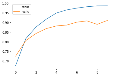
Finally, let's train the model, we'll train for 10 epochs.

history = model.fit(X_train, y_train,epochs=10,verbose=1,validation_split=0.2,batch_size=256,class_weight = class_weight)

Train on 228743 samples, validate on 57186 samples
Epoch 1/10
228743/228743 [==============================] - 97s 424us/step - loss: 8.3862 - acc: 0.6757 - val_loss: 6.4694 - val_acc: 0.7250
Epoch 2/10
228743/228743 [==============================] - 98s 428us/step - loss: 4.9663 - acc: 0.8157 - val_loss: 5.6947 - val_acc: 0.8057
Epoch 3/10
228743/228743 [==============================] - 98s 428us/step - loss: 3.0535 - acc: 0.8760 - val_loss: 4.6644 - val_acc: 0.8425
Epoch 4/10
228743/228743 [==============================] - 98s 431us/step - loss: 1.7724 - acc: 0.9164 - val_loss: 4.2003 - val_acc: 0.8679
Epoch 5/10
228743/228743 [==============================] - 99s 431us/step - loss: 1.0102 - acc: 0.9488 - val_loss: 4.4401 - val_acc: 0.8819
Epoch 6/10
228743/228743 [==============================] - 99s 431us/step - loss: 0.5970 - acc: 0.9649 - val_loss: 4.8751 - val_acc: 0.8862
Epoch 7/10
228743/228743 [==============================] - 99s 431us/step - loss: 0.4106 - acc: 0.9742 - val_loss: 4.8832 - val_acc: 0.9014
Epoch 8/10
228743/228743 [==============================] - 99s 432us/step - loss: 0.2760 - acc: 0.9815 - val_loss: 5.7314 - val_acc: 0.9080
Epoch 9/10
228743/228743 [==============================] - 99s 432us/step - loss: 0.2167 - acc: 0.9859 - val_loss: 5.8225 - val_acc: 0.8900
Epoch 10/10
228743/228743 [==============================] - 101s 440us/step - loss: 0.2202 - acc: 0.9861 - val_loss: 5.9164 - val_acc: 0.9103

plt.plot(history.history['acc'])
plt.plot(history.history['val_acc'])
plt.legend(['train', 'valid'])
plt.show()

So, we were able to get good enough performance with even a simple LSTM model. You can use the model for other types of text classification problems too.

The complete code is available at https://github.com/zabir-nabil/bangla-news-rnn

Blog

News Classification: An NLP Exercise with LSTM

Recent Blogs

DBSCAN Clustering in Machine Learning

ECG Feature extraction and Classification

Ensemble Learning in Machine Learning

Human Pose Estimation for multiple subjects with Machine Learning

Introduction to Reinforcement Learning and OpenAI Gym