In simple words, ECG represents the electrical activity of the heart and in this article, we will try to separate normal ECG patterns and abnormal ECG with the help of machine learning. We have to extract some features so that machine learning models can learn from those features. We will be using spectral moment 2, LOG, wavelength length, autocorrelation, binned entropy, sample entropy, time-reversal asymmetry statistic, and variance. We will be using multiple machine learning models to benchmark our results. Let's using SVM, KNN, Decision Tree, Random Forest, AdaBoost from the scikit-learn library. We can compare the accuracy of all the models. We will be using a 5 fold cross-validation.

ECG Feature extraction and Classification

In simple words, ECG represents the electrical activity of heart and in this article, we will try to separate normal ECG patterns and abnormal ECG with the help of machine learning.

from scipy import io, signal
import matplotlib.pyplot as plt
import dtcwt
import numpy as np
import itertools
import pywt

test_path = 'MLII/reformatted_dataset/normal/100m (0)_nsr.mat'
ta = io.loadmat(test_path)
print(ta['val'])
[[953 951 949 ... 940 943 944]]
print(ta)
{'val': array([[953, 951, 949, ..., 940, 943, 944]], dtype=int16)}
ta = ta['val']
print(type(ta))
ta.shape

(1, 3600)
print(ta)
[[953 951 949 ... 940 943 944]]
import numpy as np
ta = np.array(ta)
ta = np.reshape(ta, (3600,))

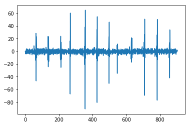
import matplotlib.pyplot as plt
plt.plot(ta)
plt.show()

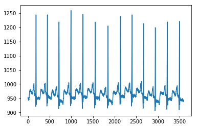
def plot_ecg(path, tit):ta = io.loadmat(path)ta = ta['val']ta = np.array(ta)ta = np.reshape(ta, (ta.shape[1],))plt.plot(ta)plt.title(tit)plt.show()

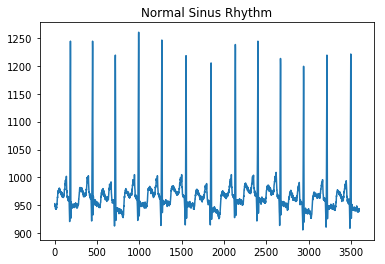
def get_ecg(path):ta = io.loadmat(path)ta = ta['val']ta = np.array(ta)ta = np.reshape(ta, (ta.shape[1],))return ta
plot_ecg('MLII/reformatted_dataset/normal/100m (0)_nsr.mat', 'Normal Sinus Rhythm')

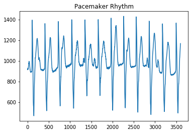
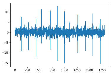
plot_ecg('MLII/reformatted_dataset/normal/107m (5)_pr.mat', 'Pacemaker Rhythm')

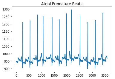
plot_ecg('MLII/reformatted_dataset/arythmia/100m (0)_apb.mat', 'Atrial Premature Beats')

from pywt import wavedec
coeffs = wavedec(x, 'db4', level=2)
cA2, cD2, cD1 = coeffs
plt.plot(cA2)
plt.show()


plt.plot(cD2)
plt.show()


plt.plot(cD1)
plt.show(

import pandas as pd
from numpy.linalg import LinAlgError
from statsmodels.tsa.stattools import adfuller
#1
def AE(x): # Absolute Energy
    x = np.asarray(x)
    return sum(x * x)


#2
def SM2(y):
    #t1 = time.time()
    f, Pxx_den = signal.welch(y)
    sm2 = 0
    n = len(f)
    for i in range(0,n):
        sm2 += Pxx_den[i]*(f[i]**2)
    
    #t2 = time.time()
    #print('time: ', t2-t2)
    return sm2




#3
def LOG(y):
    n = len(y)
    return np.exp(np.sum(np.log(np.abs(y)))/n)


#4
def WL(x): # WL in primary manuscript
    return np.sum(abs(np.diff(x)))
#6
def AC(x, lag=5): # autocorrelation


    """
     [1] https://en.wikipedia.org/wiki/Autocorrelation#Estimation


    """
    # This is important: If a series is passed, the product below is calculated
    # based on the index, which corresponds to squaring the series.
    if type(x) is pd.Series:
        x = x.values
    if len(x) < lag:
        return np.nan
    # Slice the relevant subseries based on the lag
    y1 = x[:(len(x)-lag)]
    y2 = x[lag:]
    # Subtract the mean of the whole series x
    x_mean = np.mean(x)
    # The result is sometimes referred to as "covariation"
    sum_product = np.sum((y1-x_mean)*(y2-x_mean))
    # Return the normalized unbiased covariance
    return sum_product / ((len(x) - lag) * np.var(x))


#7
def BE(x, max_bins=30): # binned entropy
    hist, bin_edges = np.histogram(x, bins=max_bins)
    probs = hist / len(x)
    return - np.sum(p * np.math.log(p) for p in probs if p != 0)
#15
def SE(x): # sample entropy
    """
    [1] http://en.wikipedia.org/wiki/Sample_Entropy
    [2] https://www.ncbi.nlm.nih.gov/pubmed/10843903?dopt=Abstract
    """
    x = np.array(x)


    sample_length = 1 # number of sequential points of the time series
    tolerance = 0.2 * np.std(x) # 0.2 is a common value for r - why?


    n = len(x)
    prev = np.zeros(n)
    curr = np.zeros(n)
    A = np.zeros((1, 1))  # number of matches for m = [1,...,template_length - 1]
    B = np.zeros((1, 1))  # number of matches for m = [1,...,template_length]


    for i in range(n - 1):
        nj = n - i - 1
        ts1 = x[i]
        for jj in range(nj):
            j = jj + i + 1
            if abs(x[j] - ts1) < tolerance:  # distance between two vectors
                curr[jj] = prev[jj] + 1
                temp_ts_length = min(sample_length, curr[jj])
                for m in range(int(temp_ts_length)):
                    A[m] += 1
                    if j < n - 1:
                        B[m] += 1
            else:
                curr[jj] = 0
        for j in range(nj):
            prev[j] = curr[j]


    N = n * (n - 1) / 2
    B = np.vstack(([N], B[0]))


    # sample entropy = -1 * (log (A/B))
    similarity_ratio = A / B
    se = -1 * np.log(similarity_ratio)
    se = np.reshape(se, -1)
    return se[0]


#16
def TRAS(x, lag=5):
    # time reversal asymmetry statistic
    """
    |  [1] Fulcher, B.D., Jones, N.S. (2014).
    |  Highly comparative feature-based time-series classification.
    |  Knowledge and Data Engineering, IEEE Transactions on 26, 3026–3037.
    """
    n = len(x)
    x = np.asarray(x)
    if 2 * lag >= n:
        return 0
    else:
        return np.mean((np.roll(x, 2 * -lag) * np.roll(x, 2 * -lag) * np.roll(x, -lag) -
                        np.roll(x, -lag) * x * x)[0:(n - 2 * lag)])
    
    
#17    
def VAR(x): # variance 
    return var(x)

from sklearn.preprocessing import StandardScaler


scaler = StandardScaler()
scaler.fit(fx)
print(scaler.mean_)
X_all = scaler.transform(fx)


print(np.mean(X_all))
print(np.std(X_all))

from sklearn.model_selection import cross_val_score
from sklearn import svm


clf = svm.SVC(kernel='linear', C=1)
scores = cross_val_score(clf, X_all, y, cv=5)
print('Accuracy: ', scores.mean(), scores.std() * 2)
Accuracy:  0.7272051167633496 0.1763962471741112
from sklearn.neighbors import KNeighborsClassifier
knn = KNeighborsClassifier(n_neighbors=100)


scores = cross_val_score(knn, X_all, y, cv=5)
print('Accuracy: ', scores.mean(), scores.std() * 2)
Accuracy:  0.7980960880559274 0.007141157066570031
from sklearn import tree
clf = tree.DecisionTreeClassifier()


scores = cross_val_score(clf, X_all, y, cv=5)
print('Accuracy: ', scores.mean(), scores.std() * 2)
Accuracy:  0.7046854082998661 0.17689499484705223
from sklearn.ensemble import RandomForestClassifier
clf = RandomForestClassifier(n_estimators=100, max_depth=None,min_samples_split=4, random_state=0)


scores = cross_val_score(clf, X_all, y, cv=5)
print('Accuracy: ', scores.mean(), scores.std() * 2)
Accuracy:  0.734374535177748 0.2567492330745884
from sklearn.ensemble import AdaBoostClassifier
clf = AdaBoostClassifier(n_estimators=10)


scores = cross_val_score(clf, X_all, y, cv=5)
print('Accuracy: ', scores.mean(), scores.std() * 2)