There are two iterations of the A3C algorithm currently in the paper: one uses a feedforward convolutional neural network, while the other uses a recurrent layer. To order to simplify it as much as possible, I must concentrate on the first one. I'm just focusing on the discrete case of action here. Maybe I'm going to write a follow-up to this including the recurrent layer as well as the expansion of continuous spaces in motion.
Asynchronous Actor-Critic Agents (A3C) in Reinforcement Learning
The A3C algorithm
Like many recent advances in deep reinforcement learning, the paper's findings were not really radically innovative algorithms, but how to push fairly well-known algorithms to work well with a deep neural network. As I will clarify in more depth in the near future, the A3C algorithm can be defined simply as using rule gradients with a function approximator where the function approximator is a deep neural network and the researchers use a clever method to try to ensure that the agent is exploring the state space well.
There are two iterations of the A3C algorithm currently in the paper: one uses a feedforward convolutional neural network, while the other uses a recurrent layer. To order to simplify it as much as possible, I must concentrate on the first one. I'm just focusing on the discrete case of action here. Maybe I'm going to write a follow-up to this including the recurrent layer as well as the expansion of continuous spaces in motion.
Pseudocode for Advantage actor-critic:
initialise parameters theta_pi for policy pi
initialise parameters theta_v for value estimate V
choose max_t (e.g. 20)
choose max_training_steps (e.g. 100 million)
choose discount factor gamma
# Update parameters once each time through this loop
for T in range(max_training_steps):
s = current state of emulator
initialise array rewards
for t in range(max_t):
sample action a from pi(a | s; theta_pi)
append a to actions
append s to states
perform action a and get new state s' and reward r
append r to rewards
s' = s
break if terminal
# Now train the parameters
R = 0
if not terminal
R = V(s, theta_v) (the estimate of the latest state)
# Compute discounted rewards
append R to rewards array
rewards = discounted(rewards, gamma)
# Compute the gradients
for each i
R_i = sum(rewards[i:])
val_i = V(s_i, theta_v)
compute grad_theta_pi log pi(a_i, s_i, theta_pi) * (R_i - val_i)
compute grad_theta_v (R_i - val_i)^2
update theta_pi, theta_v by the computed gradients
The above algorithm has the problem that the agent monitors only one part of the state space at a time and so the changes could only have a positive effect on the performance of the agent in these parts of state space while reducing the performance of the agent in other regions. Additionally, as the updates come from the agent's successive states, the updates are correlated, which is usually a bad thing for machine learning. Even in supervised learning (such as classifying images), shuffling training examples during training is a good practice to avoid correlated network updates. It can be disastrous in the context of reinforcement learning!
The authors get around this problem of correlated updates in the DQN (deep Q-learning) algorithm by using experience replay: a large buffer of all st, at, st+1,rt+1 transitions that the agent continually adds to. You sample randomly from this replay buffer during training and use these samples to make updates. It means that, as opposed to sequence transformations, you have uncorrelated transitions.
We no longer use knowledge replay with the A3C algorithm, but only use multiple agents, all navigating the state space at the same time. The idea is that the multiple agents will be in separate parts of the state space, thereby giving the gradients uncorrelated data.
That operator, implemented as described in the asynchronous document, will operate in a separate process so that the training takes place in parallel. Theta pi, theta v and the agents are updated asynchronously by a central network. This simply means that the updates are not synchronized, i.e. as soon as possible each agent updates the shared parameters.
The agent takes a copy of the shared network between each update, say theta local pi, theta local v parameters, and then executes the simulator's t max phase, working through the local policy. After t max stages, or when you see a terminal image, the agent calculates the gradients (in its own process) and then updates the parameters that are shared. If all this works in parallel, you expect the number of agents to see a linear speedup.
We can use python ray library for reinforcement learning. Let's install the libraries.
pip install tensorflow
pip install six
pip install gym[atari]
pip install opencv-python
pip install scipy
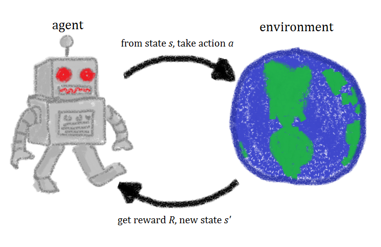
Reinforcement Learning is a field in machine learning to learn how an agent can behave in a situation to optimize some sort of aggregate reward. An agent will typically observe the current state of the environment and take action based on their observation. The action will change the environmental status and provide the agent with some numerical reward (or penalty). Then the agent will take another observation and repeat the process. State-to-action mapping is a policy, and this rule is often expressed by a deep neural network in reinforcement learning.
Each job, implemented as a Ray actor, continually simulates the environment in our A3C implementation. The driver generates a function that uses the latest template to execute several simulation phases, calculates a gradient update, and returns the update to the user. Once a task is complete, the driver must update the model with the gradient version and begin a new project with the current model.
Let's implement a ray actor to simulate the environment.
import numpy as np
import ray
@ray.remote
class Runner(object):
"""Actor object to start running simulation on workers.
Gradient computation is also executed on this object."""
def __init__(self, env_name, actor_id):
# starts simulation environment, policy, and thread.
# Thread will continuously interact with the simulation environment
self.env = env = create_env(env_name)
self.policy = LSTMPolicy()
self.runner = RunnerThread(env, self.policy, 20)
self.start()
def start(self):
# starts the simulation thread
self.runner.start_runner()
def pull_batch_from_queue(self):
# Implementation details removed - gets partial rollout from queue
return rollout
def compute_gradient(self, params):
self.policy.set_weights(params)
rollout = self.pull_batch_from_queue()
batch = process_rollout(rollout, gamma=0.99, lambda_=1.0)
gradient = self.policy.compute_gradients(batch)
"size": len(batch.a)}
return gradient, info
The manager handles employee collaboration and tries to update the requirements of the international model. The main training text appears as follows.
import numpy as np
import ray
def train(num_workers, env_name="PongDeterministic-v4"):
# Setup a copy of the environment
# Instantiate a copy of the policy - mainly used as a placeholder
env = create_env(env_name, None, None)
policy = LSTMPolicy(env.observation_space.shape, env.action_space.n, 0)
obs = 0
# Start simulations on actors
agents = [Runner(env_name, i) for i in range(num_workers)]
# Start gradient calculation tasks on each actor
parameters = policy.get_weights()
gradient_list = [agent.compute_gradient.remote(parameters) for agent in agents]
while True: # Replace with your termination condition
# wait for some gradient to be computed - unblock as soon as the earliest arrives
done_id, gradient_list = ray.wait(gradient_list)
# get the results of the task from the object store
gradient, info = ray.get(done_id)[0]
obs += info["size"]
# apply update, get the weights from the model, start a new task on the same actor object
policy.apply_gradients(gradient)
parameters = policy.get_weights()
gradient_list.extend([agents[info["id"]].compute_gradient(parameters)])
return policy